PAPERS
Transformers are RNNs: Fast Autoregressive Transformers with Linear Attention
Transformers are RNNs: Fast Autoregressive Transformers with Linear Attention
Introduction
- Transformers are currently one of the most dominant category of models being used in Natural Language Processing and also Computer Vision due to being highly effective in a varietyy of tasks.
- However, this effectiveness comes with a very high computational and memory cost. The bottleneck is mainly causd byy the global receptive field of self-attention which has a computational and memory complexity of \(\mathcal{O}(N^2)\).
- The paper introduces a linear transformer model that significantly reduces the memory footprint and scales linearly with respect to the context length. This is achieved by kernalization of self-attention and the associative proper ty of matrix products to calculate self-attention weights.
Transformers
Let \(x\in \mathbb{R}^{N\times F}\) denote a sequence of \(N\) feature vectors of dimensions \(F\). The transformer function is as follows: \(T_l(x)=f_l(A_l(x)+x)\) The function \(f_l(\cdot)\) transforms each feature independently of the others. \(A_l(\cdot)\) is the self attention function and is the only part of the trasnformer that acts across sequences. The self attention function computes for every poistion, a weighted average of the feature representations of all other position with a weight proportional to a similarity score between the representations.
The self attention function \(A_l(\cdot)\) computes for every position, a weighted average of the feature representations of all other positions with a weight proportional to a similarity score between the representations. There are 3 possible weight matrices. The attention score is calculated using 3 matrices, \(Q,K \ \text{and}\ V\) which are referred to as the "queries", "keys" and "values" respectively.
The generalized attention equation is \(V_i'=\frac{\sum^N_{j=1}\text{sim}(Q_i,K_j)V_j}{\sum^N_{j=1}\text{sim}(Q_i,K_j)}\)
Linearized Attention
- The only constraint that needs to be imposed on the similarity operator in order to it define an attention function is that it should be non-negative.
Use a kernel \(\phi(x)\) that satisfies this constraint. \(V_i'=\frac{\phi(Q_i)^T\sum^N_{j=1}\phi(K_j)^TV_j}{\phi(Q_i)^T\sum^N_{j=1}\phi(K_j)^T}\)
The summation terms will be a constant and hence can be computed just once and reused later. This gives time and memory complexity of \(\mathcal{O}(N)\)
Feature Maps and Computation Cost
- Linear attention requires \(\mathcal{O}(NCM)\) multiplications where \(C\) is the dimensionality of the feature maps and \(M\) is dimensionality of the values. This is compared to \(\mathcal{O}(N^2\text{max}(D,M))\) for softmax attention where \(D\) is the dimensionality of the queries and keys.
- The kernel used is \(\phi(x)=\text{elu}(x)+1\) where elu\((\cdot)\) denotes the exponential linear unit activation function.
Causal Masking
- The transformer architecture can be used to efficiently train autoregressive models byy maskingg the attention computation such that the $i$-th position can only be influenced by $j$ if and onlyy if \(j\leq i\).
\(V_i'=\frac{\phi(Q_i)^T\sum^i_{j=1}\phi(K_j)^TV_j}{\phi(Q_i)^T\sum^i_{j=1}\phi(K_j)^T}\)
\(V_i'=\frac{\phi(Q_i)^TS_i}{\phi(Q_i)^TZ_i}\)
- Where \(S_i\) and \(Z_i\) can be computed from \(S_{i-1}\) and \(Z_{i-1}\) in constant time hence making the computational complexity of linear transformers with causal masking linear with respect to the sequence length.
Gradient Computation
- To ensure efficieny, the gradients of the numerator are derived as cumulative sums. This allows both the forward and backward pass of causal linear attention to be in linear time and constant memory.
\(\nabla_{\phi(Q_i)}\mathcal{L}=\nabla_{\bar{V}}\mathcal{L}(\sum^i_{j=1}\phi(K_j)V_j^T)\)
\(\nabla_{\phi(K_i)}\mathcal{L}=(\sum^N_{j=1}\phi(Q_j)(\nabla_{\bar{V}}\mathcal{L})^TV_i\)
\(\nabla_{\phi(Q_i)}\mathcal{L}=(\sum^N_{j=1}\phi(Q_j)(\nabla_{\bar{V}}\mathcal{L})^T)^T\phi(K_i)\)
- The cumulative sum terms are computed in linear time and require constant memory with regard to sequence length.
Training and Inference
- When training an autoregressive model, the full ground truth sequence is available which allows parallelisation of the transformer function and attention equations. This makes transformers more efficient to train than recurrent neural networks.
- However during inference, only the current time step output is the input for the next time step, making them impossible to parallelize. Moreover, the cost per timestep for transformers is not constant and instead scales with the square of the sequence length because the attention must be computed for all previous time steps.
- The method outlined in the paper fixes this problem by making inference a constant by storing the \(\phi(K_j)V_j^t\) matrix as an internal state and updating it at every time step like a recurrent neural network.
Transformers are RNNs
- From the causal masking formulation and the training and inference discussion, it can be seen that any transformer layer with causal masking can be written as a model that give an input, modifies an internal state and then predicts an output, namely a recurrent neural network.
- The transformer equations can also be formulated as RNN equations.
\[s=0,\]
\[z_0=0,\]
\[s_i=s_{i-1}+\phi(x_iW_K)(x_iW_V)^T,\]
\[z_i=z_{i-1}+\phi(x_iW_k),\]
\[y_i=f_l(\frac{\phi(x_iW_Q)^Ts_i}{\phi(x_iW_Q)^Tz_i}+x_i)\]
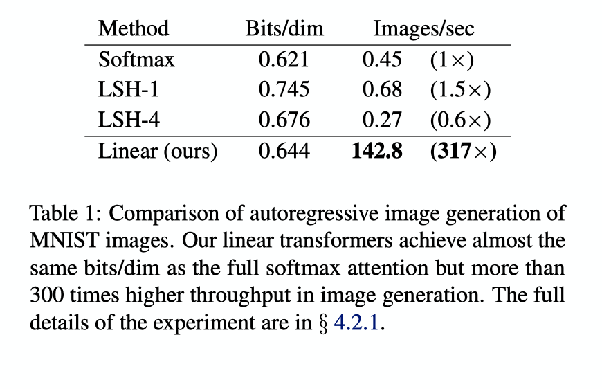
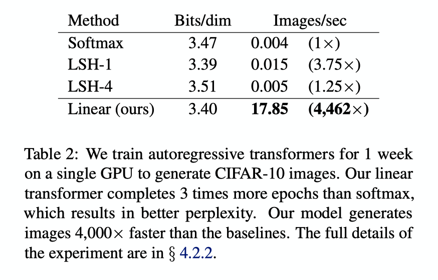
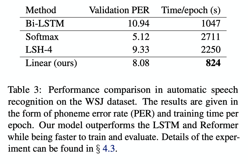
Experiments and Results